Lab 6: Potentiometric Titrations

After the lab, we should have data for pH at 0.50 mL increments of NaOH for the titration of the phosphoric acid unknown. I'm going to present a tutorial on how to get Excel to do our calculations, but I'm using the sample data used in the lab handouts, which uses different concentrations and volumes than what we actually used in the lab. This page is fairly graphics-intensive, so it may take a few moments to load.

If you need a copy of the lab handout, you can download Lab 6 (PDF, 54 KB).

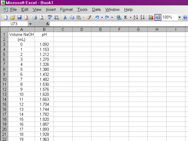
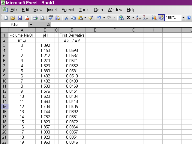
The first thing we need to do is enter our data pairs into Excel in two columns. This will probably take more time than the rest of the work with the spreadsheet combined.

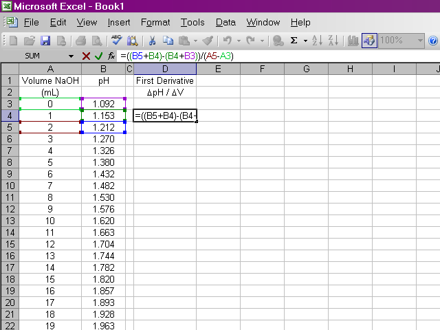
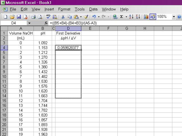
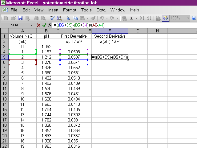
Once we have our data entered, we can calculate the first derivative of pH with respect to volume (the slope of the titration curve). A slight complication arises from the fact that if we calculate the slope between two points as rise / run, the value of the slope should be plotted at the average volume between those two points. Since it is important to know exactly how our data points relate to volume, our calculation will be slightly more involved. Essentially what we will do is take the average value of pH between the first and second and between the second and third data points and calculate the slope from those values. Highlight the appropriate cell in your spreadsheet and type the formula shown below into the formula box above the spreadsheet. Note that this first derivative value is calculated for the second volume reading and not the first. This is due to the nature in which we are averaging values of pH.

It would be repetitive and time-consuming to have to retype this formula in every cell a hundred times over. Excel will allow us to copy this formula down the column, and it will make adjustments to cell references as appropriate. Click on the box containing this newly-calculated value, and then click on the lower right corner of the box and drag it down the sheet ...

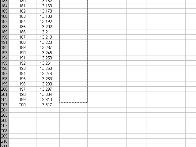
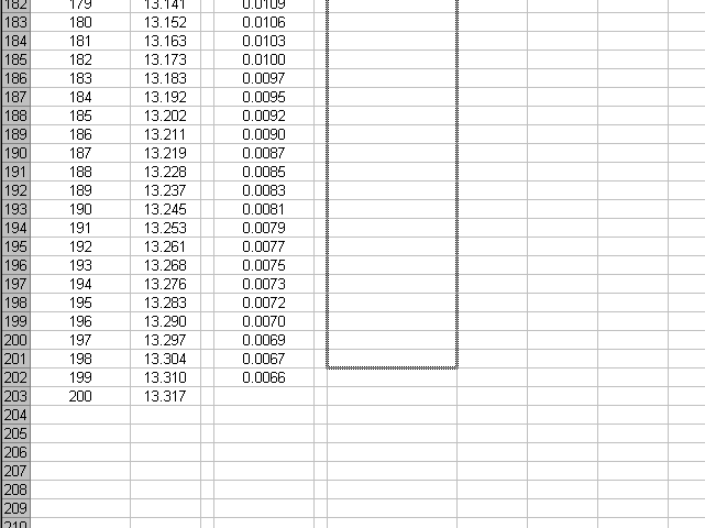
... until we reach the end of the series. Note that for the same reasons the first derivative is calculated for one data point fewer in the beginning, it will be calculated for one data point fewer at the end.

Now we have the first derivative calculated over all our data points, by writing a single formula and then copying it for the rest of the points.

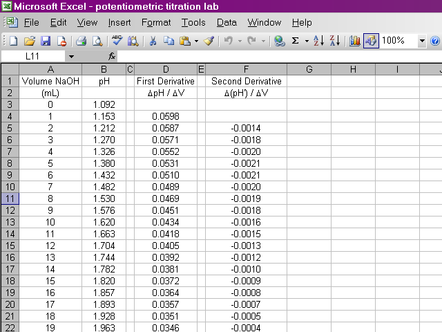
We will do something similar to calculate the second derivative, this time from the data for the first derivative and the volumes. Once again, due to the way we are performing this calculation, the second derivative will be calculated for one fewer point in the beginning.

We will copy this formula down the sheet, being careful to stop one data point short of the previous series.

Now we have calculated the second derivative for all of our data.

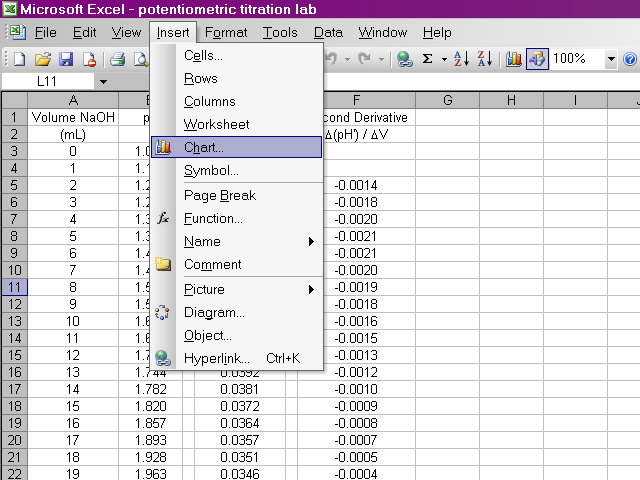
We will now begin preparing our plots. From the insert menu, select Chart.

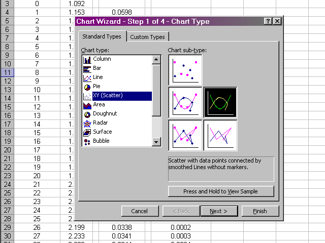
A dialog box will pop up and we will use a scatter plot. With this much data, it does not make sense to display every point, so we will have Excel connect the points with smooth lines instead. After selecting the appropriate options, click Next.

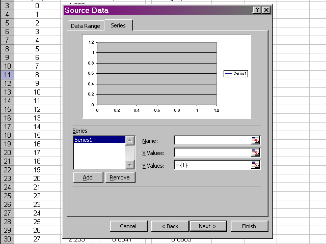
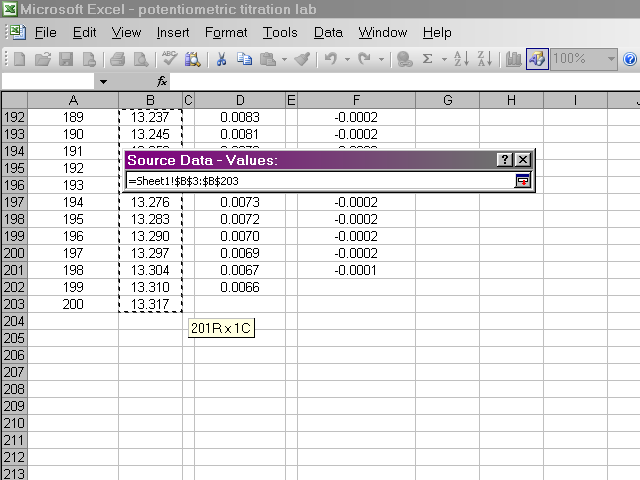
In the next pane of the dialog box, we will select the Series tab, and then select the data we wish to plot by clicking on the X Values box.

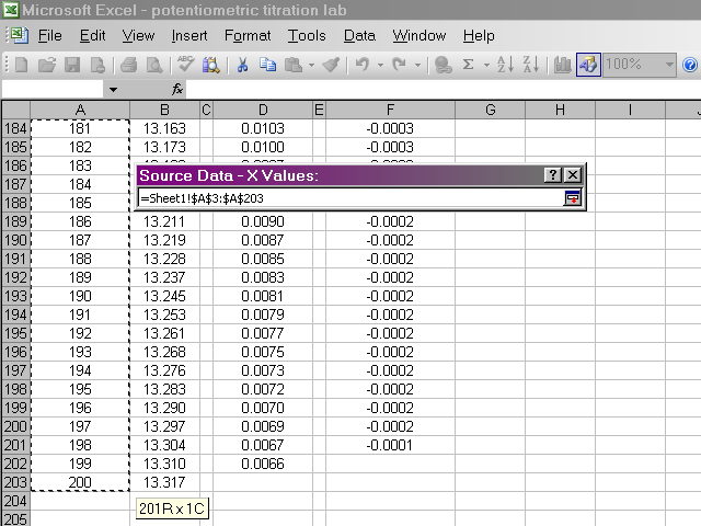
Highlight the volume data, since this is what we want to place on the X-axis, and then click back on the dialog box.

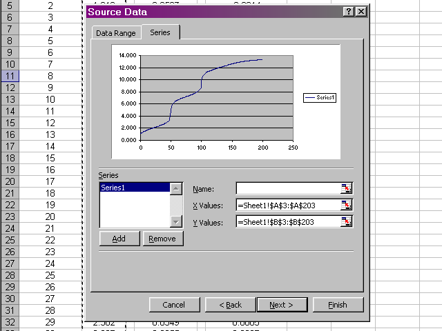
Back in the dialog box, click on the Y Values box, then highlight the pH data. Return to the dialog box.

Now we should have a preview of the data that looks like a titration curve. Click Next.

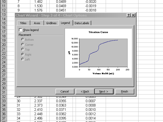
In the next pane of the dialog box, click through the various tabs to enter a title, meaningful labels on the axes, and to neaten up the plot presentation (Excel's default gridlines and legend are nonsense for what we are preparing). When all of these options have been set and you are satisfied with how the plot will look, click Next.

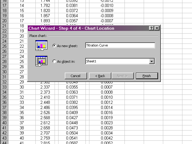
Place the new plot as a new sheet in your spreadsheet and give it a name. When you click Finish the new plot will appear.

You can get back to the data by clicking on the tab at the bottom left of the Excel window, which will be called Sheet 1 by default. In a similar fashion, prepare plots of the first derivative vs. volume and second derivative vs. volume. Be careful to select only the appropriate volume data for the subsequent plots to take into account the missing values at the beginning and end of the first and second derivative data. Your plots should have a similar appearance to the sample plots given in the lab handout.

After you have prepared the plots, take the time to format their appearance as appropriate. Some light gridlines (Right click on plot, select Chart Options to add gridlines, then right click on the gridlines and select Format Gridlines to change their appearance as appropriate) may help to enhance the readability of the plot. The scale on the axes will probably need to be adjusted (Right click on axis, select Format Axis, and change the values in the Scale tab) in order to have the data take up the entire plot without too much empty space.

At this point, you should have the plots you need to complete the data analysis as detailed in the lab handout.